Dual Sonar ESP32 Garage State Estimation

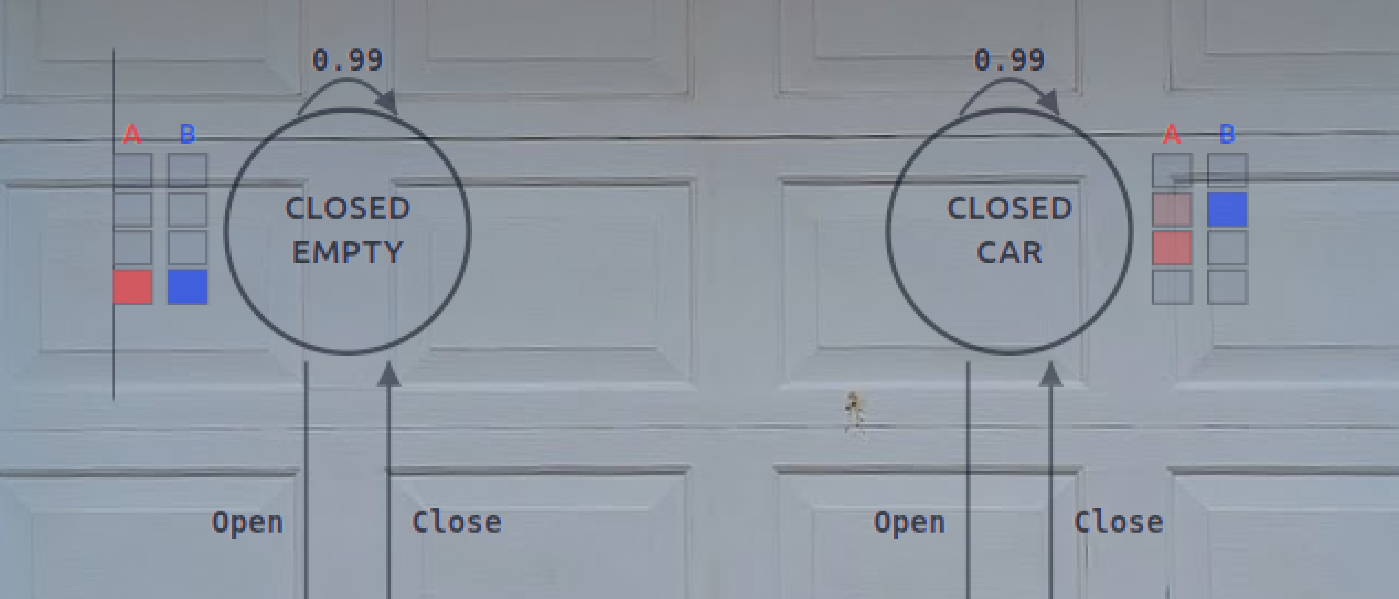
Introduction  

Part of my garage door automation project is the estimation of the state of each side of the garage. Is the garage door open or closed? Is a car present or absent?

Garage door state is great to know if you are worried you left a garage door open on leaving the house. You can check and close the door remotely if needed via the Home Assistant¹ phone app.

This summer, we had three cars commuting to work each morning. On the left side of the garage, the car that needed to leave first parked in front of the garage door. At the end of the day, that car could immediately park in front of the garage if the other was already back in the garage. Otherwise, it parked on the street until the other car returned. Being able to use a phone to check occupancy of the garage saved time from either opening the garage door to check whether a car was there, or unnecessarily parking in a temporary location.

Fortunately, after about four attempts, I finally had a reliable system.

My original post describes how I first tried contact sensors, then moved to sonar. The sonar looks down from the ceiling of your garage, and returns a different distance depending on whether it sees an open garage door rolled up just underneath, the top of a car, or the garage floor.

The problem is that sonar readings can be unreliable, particularly due to reflections from non-horizontal surfaces such as a car windshield or hood. This makes state classification by simple distance thresholding unreliable. I eventually found that a simple Hidden Markov Model² (HMM) could dramatically increase the reliability (see Garage state estimation in an uncertain world ).

Over time, however, I found that even the HMM can get confused. I found in these cases that every sonar reading fails, not just some of them. Without good data, software can’t help.

This blog post describes my solution: a second sonar further from the garage entrance, behind where the garage door rolls up. With two sonars there is a much better chance that one hits a horizontal surface such as a car roof instead of reflecting off an angled surface like the windshield or hood. Moreover, the second sonar allows the system to detect car presence even when the garage is open.

Thanks to PCBWay for sponsoring this blog post by providing the updated dual-sonar circuit boards.

Hardware Revision  

Geometry and Sensor Placement  

The physical upgrades to the system are an expanded PCB that supports four HC-SR04 ultrasonic distance sensors (two per garage door bay), and the additional sensors mounted in the garage.

On each side/bay of the garage, the sonars are positioned as follows:

• Sonar A (Door-side Sensor): Mounted near the front of the bay. When the door is closed, it measures the distance to the floor or top surface of the car. When the door rolls open, the door panels cover Sonar A, producing a deterministic short reading.
• Sonar B (Bay-side Sensor): Mounted further back along the bay ceiling, beyond the physical travel path of the open garage door. Because door panels never obstruct Sonar B, it has an uninterrupted line of sight to either the top surface of the car or the garage floor.

This dual-sensor configuration provides two main benefits:

1. Elimination of the Open-Door Blind Spot: Sonar B provides independent car-presence verification regardless of whether the garage door is open or closed.
2. Acoustic Redundancy: Ultrasonic distance sensors occasionally report maximum-range error timeouts or reflection jumps. Even if one sensor suffers failed or noisy readings, the statistical weight of the second sensor helps maintain state stability.

PCB update  

Fortunately, the ESP32 has plenty of GPIO pins for supporting additional sonars. In previous board updates, I found that Google Gemini can help update my KiCAD schematics for changes like this, check GPIO pin assignments, and also help update firmware to reflect the updated board. It isn’t perfect: I still had to make corrections, but these systems are improving quickly. I manually made the necessary layout changes in KiCAD, resulting in a slightly larger board to accommodate the additional connectors.

I uploaded my Gerber files to PCBWay. I like to use the “Quick Order” option, starting with the Gerber file upload, so most of the options like board size or number of layers are automatically supplied. As usual, I selected “HASL lead free” and ordered a non-framework stencil with the smallest possible size .

An annotated picture of the PCB populated by SMD components, before soldering the through-hole components such as connectors and relay modules, is shown below.

Almost no difference in cost  

There is no real difference in the cost of PCBs with extra connectors for two more sonars, and HC-SR04³ sonars are currently available from AliExpress for less than a dollar apiece. The total hardware expense of the system remains extremely low. The main cost for the dual sonar deployment is the extra time required to site, wire, and aim the additional sensors.

Firmware update: Expanding the State Space and HMM Firmware  

In the original single-sonar model, the system tracked three hidden states (DOOR_OPEN, CAR_PRESENT, and GARAGE_EMPTY). With two sensors per bay, we expand our model to four distinct hidden states:

• DOOR_CLOSED_EMPTY
• DOOR_CLOSED_CAR
• DOOR_OPEN_EMPTY
• DOOR_OPEN_CAR

Multi-Observation Viterbi Algorithm  

To process readings from both sensors, we updated our ESP C++ firmware to evaluate a multi-observation Hidden Markov Model.

Assuming that the acoustic noise of Sonar A and Sonar B are conditionally independent given the true hidden state $S$ , the probability of observing reading pair $(O_A, O_B)$ is the product of their individual values:

In the firmware, each garage bay has two emission matrices:

• Matrix $E_A$ : Maps distance buckets from Sonar A to state probabilities.
• Matrix $E_B$ : Maps distance buckets from Sonar B to state probabilities.

During each two-second sampling loop, the ESP32 updates its estimate of the current garage state based on new sonar readings $d_A, d_B$ :

1. Measurement Quantization: Quantizes distances $d_A, d_B$ into observation bins $O_A, O_B$ .

   💡 Convert each distance in meters to an integer representing one of a few possible meanings such as “very close”, “near”, “medium”, “floor-distance”, or “very far”.

2. Joint Emission Evaluation: For each potential state $j$ , computes the joint emission probability: $$P(O_A, O_B \mid S_j) = E_A[j, O_A] \times E_B[j, O_B]$$

   💡 “Given a potential garage state such as DOOR_CLOSED_EMPTY, how likely are we to see this specific pair of sonar readings?”

3. Viterbi State Update: Runs the standard Viterbi⁴ update step to compute the updated probability for each state and select the most likely current state.

   💡 “Combining physical state transitions with the new sonar data, how likely is each state now, and which should I report as the actual state?”

Sonar configuration, and training models  

Two more steps are necessary to make the system work:

1. Position the sonars in the garage. The sonars should ideally be placed over the bay’s central axis to avoid seeing the sides of the car, and point straight down. Their line of sight should be free of obstructions. This is easier in some garages than others. Test the sensor readings and adjust mounting as needed.
2. Collect training data, and train the HMM. In my previous post I discuss how I save sonar readings to InfluxDB, browse the data in Grafana, and download representative data for each garage state for each side of the garage. I built a training set from the downloaded data, train HMM models for each side of the garage, and upload these HMM models to the device through its web interface.

The latter step requires some infrastructure and specialized effort. It is difficult for others to replicate at this time, so needs to be made easier somehow.

Result: Unambiguous Detection and Noise Rejection  

With well-positioned sonars and properly trained models, the system reports the state of the garage reliably and correctly.

A common case where the two sonars make a difference is where one is seeing reflection off a windshield or hood. In these cases of reflection, measured distance may vary greatly depending on air temperature. In the case shown below, a car remains present in the left bay the entire time (a little more than a day), and the door is closed except for half an hour near the end of the period. The car is facing the front of the garage, so the door-side sonar sees the angled windshield. As air temperature falls from near 50℃ in early afternoon (sun on the roof of the garage!) to 30℃ in early morning, the door-side sonar reading drifts from a noisy 2.5m to 8.5m. Because the rear sonar clearly sees the roof of the car the entire time, and the front sensor clearly sees the garage door 0.4m below when it is open, the HMM remains certain and correct about the state of the garage.

On the right side, the garage starts closed and empty. The garage door is later opened, a car enters facing inward, then the door is closed. When the bay is empty, the rear sonar has trouble seeing the floor, so noisy readings vary from the near correct 3m to around 6m. The front sonar, however, cleanly reads the distance to the floor, then the garage door, and finally the roof of the car. The rear sonar does see the roof of the car when present.

In both cases, the HMMs manage the stochastic nature of the readings, and correctly report the state of the garage to Home Assistant without any “state chatter”.

Conclusion  

By adding a second sonar for each garage bay, and upgrading firmware to support multi-observation HMMs, I finally achieved reliable and correct estimation of both car occupancy and garage door state. Moreover, occupancy can be determined even when the door is open. The ESP32 easily handles the computation, and the extra hardware cost is negligible.

The updated PCB schematics, OpenSCAD project box and sonar mount designs, and the C++ firmware are available as always at the Garage133 GitHub Repository .

References