Garage state estimation in an uncertain world

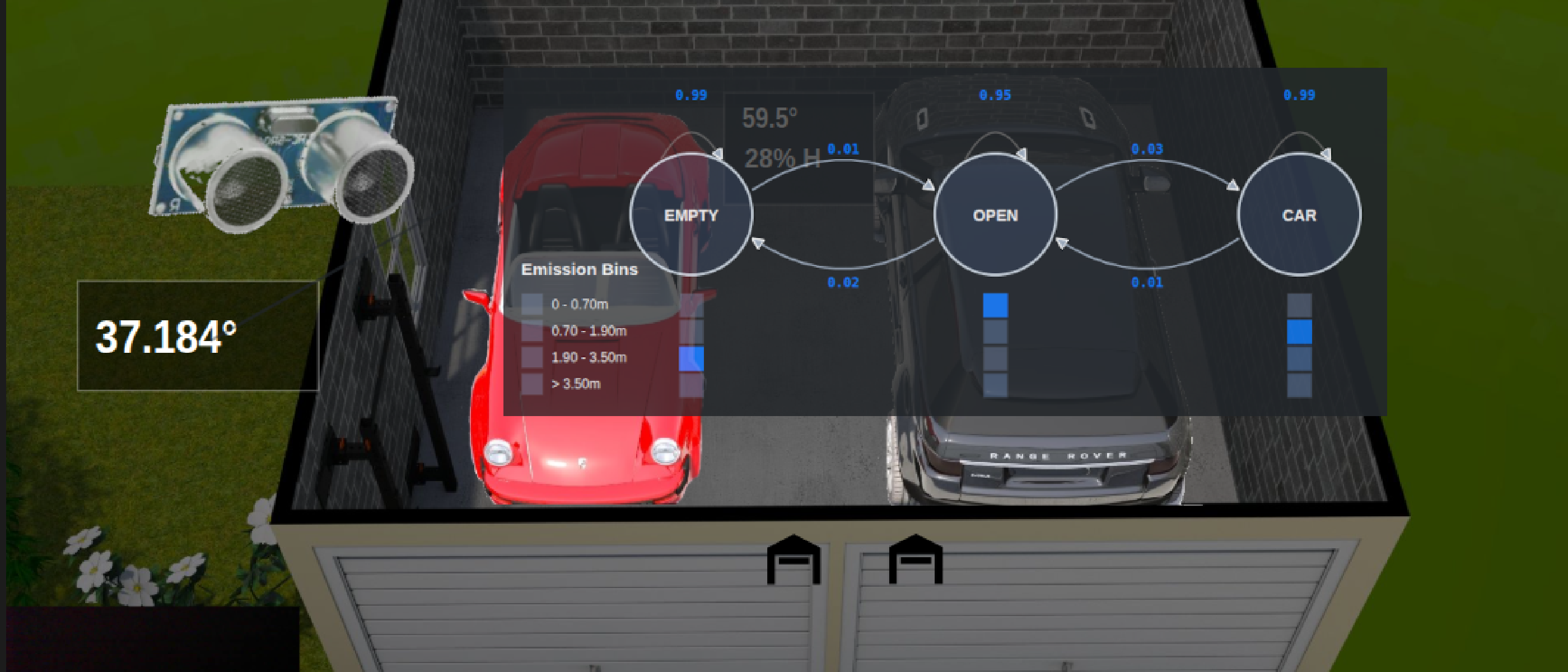
Introduction  

I built a device I call Garage133 (see my earlier post) to control our garage doors and monitor the state of the garage. For each side, a sonar sensor determines whether the garage door is open or closed, and whether a car is present. This allows our home automation system to alert us if a door is left open and provides the capability to close it remotely.

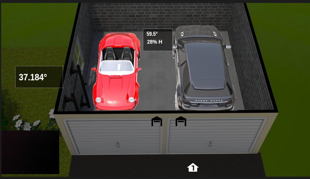
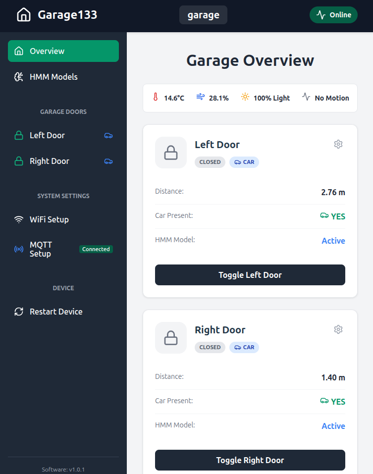
The image above shows the estimated garage state as rendered in our live Home Assistant¹ dashboard using the FloorPlan² card. The rendering includes door status, car presence,³ temperature, humidity, motion, charging, etc…

Garage133 basically works well. All we really need is an easy way to open and close the garage doors without overpaying for a closed, cloud-based system like MyQ⁴, and we have that. But the state detection logic proved surprisingly difficult to get right. This post explores why this is—the nature of sonar—and how we solved it using Hidden Markov Models.

The Challenge: Sonar is Stochastic  

Using distance measurements to detect garage state is straightforward, at least in theory. A sensor looking down from the ceiling should detect one of three surfaces:

• The garage door rolled up directly under the sensor,
• The roof or hood of a car, or
• The garage floor.

Even with reliable measurement, results for a given state will still vary. Cars are never parked in the exact same spot, and the floor can be cluttered. But the real problem is that sonar sensors do not provide perfect measurements.

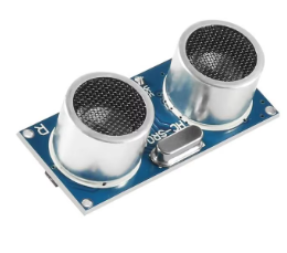
In many ways, sonar is an ideal choice for this environment. The sensors are inexpensive, easy to integrate, and have proven remarkably durable across wide temperature and humidity ranges. I use the ubiquitous HC-SR04⁵ sensors, which are readily available for just a few dollars.

The difficulty is the physical nature of sound waves. Ultrasonic waves reflect off smooth, angled surfaces like a car hood as if they were mirrors. When this happens, the sensor doesn’t receive a return from the target surface. Instead, it detects whatever surface is “visible” in the reflection, such as the garage door or a far wall. This results in a measurement significantly longer than the true distance.

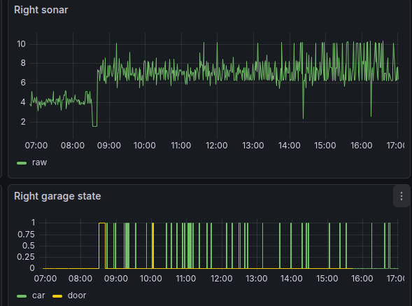
Sometimes the signal doesn’t return at all, causing the sensor to report a maximum-range “error” value (e.g., 12m). In a static configuration, sonar readings often alternate between the true distance, a long reflection, and no return at all. We aren’t dealing with a simple distance; we are dealing with a stochastic set of readings over time.

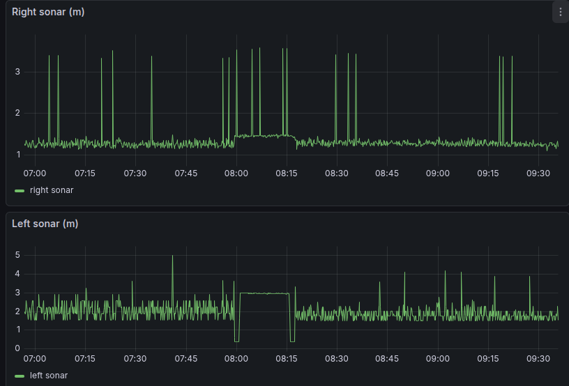
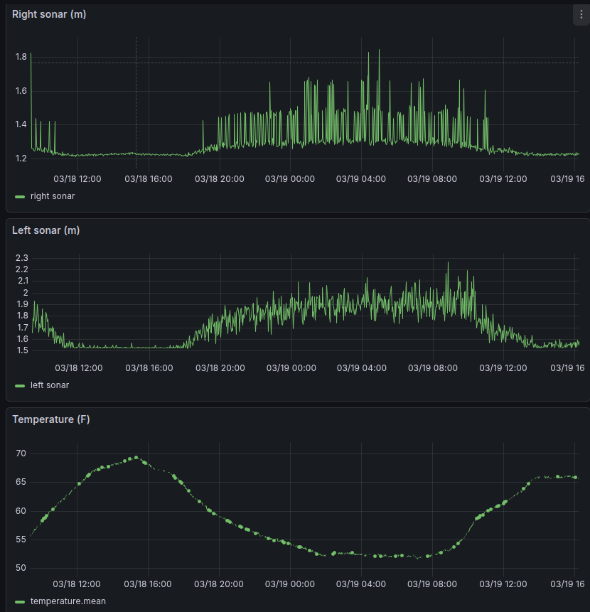
As shown above, readings in the “door open” and “empty” states are relatively clean, while the “car present” state is very noisy. Readings on the right side of the garage are not independent of the state of the left. Furthermore, as shown below, sensor noise can vary dramatically with temperature.

The Initial Solution: Simple Thresholds  

My first attempt at classification relied on simple distance-based rules. Given the garage geometry, I mapped measurements directly to states:

• < 0.1m: Error (Ignore)
• 0.1m to 0.7m: Door Open
• 0.7m to 2.4m: Car Present
• 2.4m to 4.0m: Garage Empty
• > 4.0m: Error (Ignore)

This approach was fragile. If a reflection caused a 1.5m reading to jump to 3.0m, the reported state would immediately flicker from “Car Present” to “Empty.”

While these problems can be mitigated using smoothing and outlier rejection, tuning these magic numbers is a frustrating exercise that only mostly works.

HMMs: A Simple Probabilistic Solution  

To solve this, I needed a model that looks past individual data points to estimate the most likely underlying state. While a neural network could learn this behavior, it is a “black box” that is difficult to debug and overkill for an ESP32.

Instead, I chose to use Hidden Markov Models (HMMs)⁶. An HMM is a classic probabilistic tool designed specifically for this “noisy observation” problem. HMMs are computationally cheap, mathematically transparent, and remarkably effective for state estimation. Originally described in the 1960s, HMMs powered early speech recognition systems starting in the 1970s. While the complexity of human speech strained the model’s capabilities (today’s systems using neural nets are vastly superior), the garage classification problem is much simpler and well within an HMM’s strengths.

Hidden States vs. Observations  

An HMM distinguishes between what we can measure (the Observations) and the physical reality we want to know (the Hidden States).

In our case, the hidden state has three values: DOOR_OPEN, CAR_PRESENT, and GARAGE_EMPTY. The observations are the sonar readings, which we group into discrete “buckets” (Near, Mid, Far, and Out-of-Range).

The HMM is defined by three probability sets:

1. Initial State: The “best guess” when the device first boots.
2. Transition Probabilities: The physical likelihood of moving between states. (e.g., You cannot transition from EMPTY to CAR without the door being OPEN).
3. Emission Probabilities: The likelihood of a specific reading given a state. (e.g., A CAR state mostly emits “Mid”-distance readings, but has a known probability of emitting “Far” readings due to reflections).

After each measurement, the device updates its estimate using the Viterbi Algorithm⁷. Because the model understands both physical constraints (transitions) and sensor behavior (emissions), it resists state estimation flickering. A single noisy reading might nudge the probability only slightly, but a consistent sequence of observations can change the reported state.

Gathering Training Data  

State updates are usually sent to Home Assistant via MQTT just once per minute. This is far slower than the underlying two-second measurement cycle. Training the HMM requires a dataset collected at this higher rate.

Leveraging the UDP Logger  

The Garage133 firmware includes a UDP-based logging side-channel that broadcasts text messages with each sensor reading. I updated a Python receiver (esplog) in my home lab to parse these raw metrics and forward them to an InfluxDB instance.

Here is an example of the messages parsed by this system:

1.510 m 8873 usec | 1.212 m 7122 usec | 60.1 degf

This pipeline provides the high-resolution data necessary for training.

Building the Training Set  

I built a data curation toolkit in Python to transform these raw logs into a labeled dataset:

1. Download: Fetch raw sonar sequences from InfluxDB.
2. Trim & Label: Use an interactive tool to mark “episodes” where the state was known (e.g., “The car was present from 8:00 PM to 7:00 AM”).
3. Train: Run the HMM training script to calculate the emission probabilities for each side of the garage.

The training process is surprisingly simple. I hard-code the initial state and transition probabilities based on rough estimates of garage usage. The model only needs to learn the emission patterns—the statistical distribution of sonar readings for each state. On my training set (yes, I should have a separate evaluation set), this approach achieved 100% accuracy for the left door and 99.8% for the right.

If ever the model performs poorly, I can download the data from that time span, supply the correct labels, and update the training set.

ESP32 Implementation  

The resulting inference engine is a lightweight C++ class. Every two seconds, the ESP32 performs three constant-time steps:

1. Bucketing: Maps the raw distance to an observation bin.
2. Update: Executes the Viterbi step to update the belief of each hidden state.

This logic uses negligible memory and CPU time compared to the device’s other tasks. The most likely state is then pushed to Home Assistant, resulting in a reliable classification that is nearly immune to sensor flicker.

Real-Time Visualization with Svelte  

Along with the new HMM classification system, this update of Garage133 adds a Svelte-based web interface (see Building a Modern ESP32 Web Interface with Svelte and AI). The new dashboard supports uploading HMM parameters as JSON files directly through the browser without reflashing the firmware.

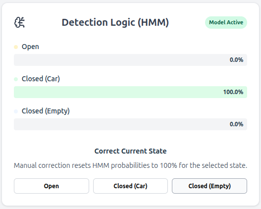
The interface also provides a “View Probabilities” tab. You can see how certain the model is of the current state and watch probabilities update in real time in response to activity in the garage.

Conclusion  

Applying a Hidden Markov Model transforms noisy sensor readings into a reliable estimation system. Using an “old school” inference method keeps the system easy to interpret, debug, and run on a constrained device like the ESP32.

References